A Categorical Can of Worms III

Examining categorical interactions in logit models using Marginal estimates and Marginsplot

Kevin Ralston 2018, York St John University

Introduction

This post is the third in a series of blogs which examine parameterisations of interactions in logit models. The first post outlined the generic, ‘conventional’ approach to including categorical interactions in logit models. The second post outlined an alternative specification of a categorical interaction in a logit. The current post outlines the application of marginal estimates and the marginsplot graph in the examination of categorical interactions in logit models.

Marginal estimates

Marginal estimates of categorical data are now part of the standard tool box in sociological research outputs. Margins produce estimates which have a ready interpretation. This is helpful because, as we have seen, working out what a model is showing us when an interaction is included is not straightforward. Williams (2017) explains what a marginal probability shows us in a logit model:

In the logit marginal results report the probability that a category is in the category coded 1 on the outcome. The MEM [marginal effect at means] for categorical variables therefore shows how P(Y=1) changes as the categorical variable changes from 0 to 1, holding all other variables at their means.

quietly logit class3 i.sex##i.ft i.qual c.age
margins i.sex#i.ft,

To produce marginal estimates at means we will estimate the basic model we have specified previously. We then follow this with a new line of code which includes the margins command, along with the variables included in the interaction. The quietly command here tells Stata not to produce the output for the model (we’ve seen it already).

Table1, Stata output, marginal estimates at means for an interaction from a logistic regression modelling membership of social class III, including independent variables sex, has a qualification, working full-time or part-time and age, also an interaction between age and working FT/PT. Source is GHS 1995, teaching dataset

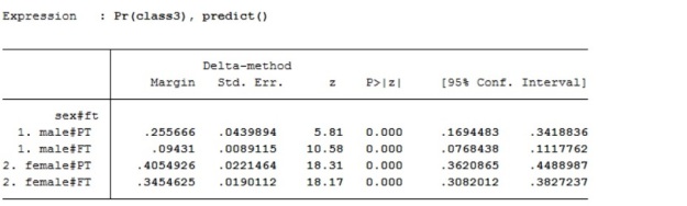
In this case the margins are interpreted as the probability that each of the categories is in social class III at the average value (mean) of the other variables included in the model.

A standard criticism of marginal estimates at means is that the average value at which the estimates are calculated may have no substantive meaning. For example this model includes a categorical measure of whether an individual has qualifications, or not. By coincidence this variable is balanced close to 50% in each category. In a model including say, 30% with no qualifications the average marginal probabilities would be computed for an individual with 30% no qualification. In this model the margins are for an individual with ~50% no qualifications. This is problematic because we are referring to discrete categories. Someone with 50% no-qualifications cannot exist.

quietly logit class3 i.sex##i.ft i.qual c.age
margins i.sex#i.ft, at(qual=1) post,

It is also possible to estimate the marginal at a specific value of independent variables, such as qualifications. These have been described as adjusted predictions or predictive margins. This may be preferred. This is the specification I prefer as it offsets the criticism made above. It does not however mean that anyone in the data necessarily occupies the combination of categories in the model. There may still be no part time male workers with no-qualifications at the mean age of the sample. If there were we would expect them to have a probability of occupying social class III of .178 (quite low, closer to 0 than 1).

Table2, Stata output, adjusted predictions for an interaction from logistic regression modelling membership of social class III, including independent variables sex, has a qualification, working full-time or part-time and age, also an interaction between age and working FT/PT. Source is GHS 1995, teaching dataset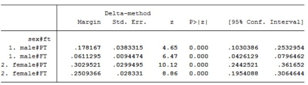

Marginsplot

The margins command has a neat graphing functionality.

Figure1, is a graphic of the marginal probability at means of being in social class III for the working full-time, part-time and sex interaction. The code for this is reported below.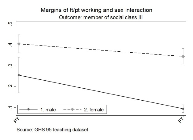

logit class3 i.ft##i.sex i.qual c.age

       margins i.ft#i.sex,

             marginsplot , name(g2, replace) scheme(s1mono) ///

                    title (“Margins of ft/pt working and sex interaction”) ///

                    subtitle(“Outcome: member of social class III”) ///

                    legend(pos(7) ring(0)) ///

                    xtitle(“”) ytitle(“”) ///

                    xlabel(,angle(45))  ///

                    caption(“Source: GHS 95 teaching dataset”)   

 

To produce this graph you might notice I switched the position of the ft and sex dummy variables in the model. The graphical specification seems more sensible depicting ft/pt on the x-axis and depicting the difference within and between men and women. Maybe I should switch all the models so they are consistent. I had originally included sex in the model first for two reasons. Firstly, people have a biological sex and a socially constructed gender which influences their experience and choices, before they have a full time or part time job. Secondly, gendered occupational segregation is the area of substantive interest.

Building an analysis is an iterative process. There are good reasons to include sex before ft in the model, but in this case the interaction is presented more sensibly when organised i.ft##i.sex. Constructing an analysis often involves making small decisions and trade-offs like this.

Conclusion

In conclusion, I would suggest anyone fitting categorical interactions in logit models should both apply and report the marginal estimates. These have ready and relatively straightforward interpretations. They are certainly more intuitive than the interpretation of the results of a categorical interaction output in Stata applying a conventional interaction in a logit model.

Suggested reference should this post be useful to your work:

Ralston, K. 2018. A categorical can of worms III: Examining categorical interactions in logit models using Marginal estimates and Marginsplot. The Detective’s Handbook blog, Available at: thedetectiveshandbook.wordpress.com/2018/10/15/a-categorical-can-of-worms-iii/[Accessed: 15 October 2018].

 

Stata 15 Dynamic Documents: ‘.do files on steroids’

Roxanne Connelly, University of Warwick

Currently the transparency of social science research is poor, particularly in sociology. We tend to place little emphasis on undertaking research in a manner that would allow other researchers to repeat it, and approaches to sharing details of the research process are ad hoc and rarely used. To improve the transparency and reproducibility of sociological research I believe a step-change is required, not only the way we present the results of our research, but in the research process. Producing documentation for replication throughout the research process seems to be a key way in which we can move transparency from being an afterthought in the research process to being front and centre in our research conduct.

Building research transparency into the research process is not new, and borrows from the principles of literate programming introduced by Knuth (1992) in the field of computing science. Literate programming involves the weaving of narratives directly into live computation, interleaving text and documentation (beyond simple comments) with code and results to construct complete and transparent computations. The goal is to explain to humans, rather than machines, in natural language, what processes are being undertaken. The idea of literate programming has been taken up within the scientific computing community as a means to share self-documenting reproducible workflows but is very rarely implemented in sociology.

There are some packages available that can facilitate this type of literate programming for social science research. A notable example is Jupyter Notebooks, a web-based application that supports literate programming in a wide variety of languages (over 50 at present), including data analysis languages widely used for longitudinal social science research (i.e. R and Stata). Jupyter notebooks can run code from different computer programs in a language agnostic environment and can incorporate text and images. These notebooks can be shared and researchers can re-run the notebook and examine the results for themselves. An introduction to Jupyter Notebooks is available here. I am a big fan of Jupyter Notebooks, but currently an important drawback of this application is that it is difficult to install and there is a steep learning curve to get it working, particularly for those of us with limited computing science skills.

There are other packages available within specific statistical computing software environments that allow the combination of code, outputs and free text, e.g. Markdown and KnitR within R, or MarkDoc and Weaver in Stata. My main package is Stata so I was very excited to hear that their latest release (Stata 15) incorporates the capacity to create dynamic documents using Markdown. This allows you to mix Markdown with Stata commands and create a document that interweave the commands, output and text. Stata describes this as ‘a do-file on steroids.’

This blog provides an initial demonstration of Stata’s dynamic documents in action, and may serve as a useful start-up guide for some. I may add another blog once I have used it for the complete workflow of a real piece of data analysis. Here I describe the use of dyndoc which turns a plain text document into an HTML document, there is also putdocx (to create word documets) and putpdf (to create PDF files) but I have not looked at these yet.

Using dynamic documents is straightforward. First you create a plain text file containing the text you want to contain in the document along with the code. This file can include standard Markdown to create text formatting (e.g. bold, italics). When you have completed this file you run the dyndoc command (shown below) and your plain text file will be converted into an HTML document. You could then convert this to a PDF document using an HTML to PDF converter.

. dyndoc filename.txt, replace

To incorporate Stata code and output you use ‘tags’ in the plain text file which indicate whether the commands should appear in the document or not, or whether the output should appear in the document or not. To get the document formatted nicely you need to download the stylesheet ‘stmarkdown.css’ and the file ‘header.txt’ and save them in your working directory.

Here is my plain text file: blogexample

Here is the file that is produced by dyndoc (saved as a pdf to post): blogexamplehtml2pdf

I am really impressed with dyndoc, it was super quick to learn and provides a really straightforward way to improve the reproducibility of your work. Right now I anticipate that I will use it to create a document that can be attached as supplementary materials to journal publications. A dyndoc would greatly surpass a log file or .do file as a reader friendly way to present the complete workflow of a piece of research. Of course the effectiveness of a dyndoc for enabling reproducibility also requires the researcher to put the work in to provide sufficient annotation and description throughout the file. But if the dyndoc is cultivated throughout the research process this could be relatively painless.

There may be more eloquent ways to make use of dynamic documents in Stata and I am sure I will pick up more tricks as I use this more. I welcome comments from more experienced users of dyndoc!

Quantitative Methods Pedagogy in Sociology: What have we got to go on?

Kevin Ralston, University of Edinburgh, 2015

A systematic review of the social science research methods pedagogy literature, taken over a decade, turned up 195 papers (Wagner et al., 2011). The review concluded that there is no pedagogical culture underlying the teaching of research methods in social science. Given that this conclusion is applied to social science as a whole, taking one of the disciplines and then focussing on just quantitative methods (QM) pedagogy is unlikely to result in a different conclusion. Indeed I have similarly surveyed the sociology QM pedagogy literature, taking a 25 year period, and cannot disagree with the finding of Wagner et al. (2011).

Over parallel timescales there have been several pushes to increase the level and capacity of QM teaching in UK social science – to name some: there is the Q-Step programme (http://www.nuffieldfoundation.org/q-step); the evolution of the ESRC Doctoral Training Centres; the AQMeN initiative to build quantitative methods capacity (https://www.aqmen.ac.uk/); the British Academy’s ‘Count us in’ report and suggested approach to a data skills strategy (www.britishacademy.ac.uk/countusin). The intentions here a laudable. Concepts such as methodological pluralism are cited (Payne et al., 2004) and any discipline which does not have all the available tools at its disposal is, in principle, weaker for it. In a note of optimism Kilburn et al. (2014) suggest that the policy foregrounding of the importance in methods in social science, together with the ‘capacity building’ policy rhetoric, may lead to an increased emphasis on pedagogy. What it means, however, to have a policy to build methodological capacity, in subject areas where there are little meaningful, evidenced, pedagogical approaches to teaching practice, is an open question.

Despite its paucity, there are the grass roots of literatures in sociology which could potentially grow into dynamic and fertile pedagogical fields. One of the themes in the literature advocates or describes general approaches to QM teaching. These are often articles written from experience (someone who has taught the subject area for many years) or suggesting how things are done within an institution (this is how we/I do it here) (e.g. Atkinson et al., 2006; Auster, 2000; Fischer, 1996; Lindner, 2012; Strangfeld, 2013). This is a useful resource. We cannot simply discount the views of a professor who has spent a career teaching in the field. Similarly, a description of how an institution programs QM teaching may very well give an example of best practice. Although it is useful for the field to build this information up it is not a substitute for an empirically informed pedagogy. There is an element of received wisdom associated with this literature.

The empirical literature researching QM pedagogy in sociology is limited but begins to give us something to go on. Typically these studies cover a year in a course or an institution (Delucchi, 2014; Maltby, 2001; Murtonen et al., 2008; Murtonen and Lehtinen, 2003; Wills and Atkinson, 2007). There is also a stream in the published work which assess an intervention in a course where, perhaps, a new mode of teaching or gimmick is tried (e.g. Delucchi, 2007; Schumm et al., 2002). The studies are often not too rigorous and may be based on small class sizes, n <100 (e.g. Maltby, 2001; Murtonen and Lehtinen, 2003; Pfeffer and Rogalin, 2012). Although, there are instances of larger studies where research has been done at institutional or departmental level, or over several years of teaching (Wilder, 2009; Williams et al., 2008). Often the evaluation is based upon student feedback (e.g. Auster, 2000) rather than building an experimental design to test the teaching practice (e.g. Raymondo and Garrett, 1998; Smith, 2003). It would be unfair to be over critical of this small literature. The work has limitations, however these studies are the only attempts to move towards generating an evidence base for our QM teaching practice. Despite weaknesses, this work is, in a sense, pioneering, and represents time taken to engage in an unfashionable but important field. This research provides a foundational contribution to the subject area.

Debate over the concept of student anxiety about statistics within social science encapsulates the issue of incomplete evidence conflating with received wisdom. The belief that social science undergraduates are apprehensive about their studies related to maths, statistics, and quantitative methods in general, is often cited in literature (e.g. Bridges et al., 1998; Paxton, 2006; Schacht and Stewart, 1990). The concept of maths anxiety is not exclusive to social science, it is also seen as a problem within specifically numerate subjects too (Henrich and Lee, 2011).  DeCesare (2007) suggests the concept to be overstated, showing that 40% of sociology students in a single institution, who responded to a survey in the U.S., report no angst. Williams et al. (2008) similarly found only a slight majority to report angst in a sample of students in England and Wales. Some work has been undertaken comparing anxiety between academic fields. In limited study comparing social science, health science, arts and hard science students Hamza and Helal (2013) found no significant differences in the mean level of maths anxiety. However, a comprehensive comparison of the level of anxiousness, both, between social science disciplines, and between social science and more numerate subjects, has yet to be undertaken. In the absence of a study of this nature, we do not know whether social science students are significantly more ‘frightened’ of numbers than their more numerate counterparts or whether some social sciences are faring better than others in this respect.

Moving the discussion on statistical anxiety amongst social science students towards an evidential basis is necessary if we are to address it. If it is the case that there is little difference in levels of anxiety between subjects then perhaps it is time to move beyond the anxiety definition which could itself be unhelpful in acting as a kind of self-fulfilling prophesy (DeCesare 2007). By the same token, if there really is an excessive angst in certain social sciences then we need to employ clear targeted strategies to address this, strategies based on evidenced pedagogy. At the moment, as a set of disciplines, it is uncertain whether social science is a special case of math anxiety, or, what can be implemented which is shown to reduce the level of worry associated with the study of maths in relation to social science.

Until we have an evidenced understanding of what constitutes good practice in QM teaching how do we know whether we are really improving capacity? Engendering an evidenced QM pedagogical practice for social science is a large proposition. It requires a generation of researchers interested and incentivised which would bring the production of research and literature to a critical mass. This could then be sustained by the availability of funding into developing QM teaching. Unless we achieve a reflective, verifiable, pedagogical culture, it is questionable how successful the aim of capacity building can be.

References

Atkinson, M.P., Czaja, R.F., Brewster, Z.B., 2006. Integrating Sociological Research Into Large Introductory Courses: Learning Content and Increasing Quantitative Literacy. Teach. Sociol. 34, 54–64. doi:10.1177/0092055×0603400105
Auster, C.J., 2000. Probability Sampling and Inferential Statistics: An Interactive Exercise Using M&M’s. Teach. Sociol. 28, 379–385. doi:10.2307/1318587
Bridges, G.S., Pershing, J.L., Gillmore, G.M., Bates, K.A., 1998. Teaching quantitative research methods: A quasi-experimental analysis. Teach. Sociol. 26, 14–28. doi:10.2307/1318676
DeCesare, M., 2007. “Statistics anxiety” among sociology majors: A first diagnosis and some treatment options. Teach. Sociol. 35, 360–367.
Delucchi, M., 2014. Measuring Student Learning in Social Statistics: A Pretest-Posttest Study of Knowledge Gain. Teach. Sociol. 42, 231–239. doi:10.1177/0092055×14527909
Delucchi, M., 2007. Assessing the impact of group projects on examination performance in social statistics. Teach. High. Educ. 12, 447–460. doi:10.1080/13562510701415383
Fischer, H.W.I., 1996. Teaching Statistics from the User’s Perspective. Teach. Sociol. 24, 225–230. doi:10.2307/1318815
Hamza, E., Helal, A.M., 2013. Maths Anxiety in College Students across Majors: A Cross-Cultural Study. Educationalfutures 5.
Henrich, A., Lee, K., 2011. Reducing Math Anxiety: Findings from Incorporating Service Learning into a Quantitative Reasoning Course at Seattle University. Numeracy 4. doi:http://dx.doi.org/10.5038/1936-4660.4.2.9
Kilburn, D., Nind, M., Wiles, R., 2014. Learning as Researchers and Teachers: The Development of a Pedagogical Culture for Social Science Research Methods? Br. J. Educ. Stud. 62, 191–207. doi:10.1080/00071005.2014.918576
Lindner, A.M., 2012. Teaching Quantitative Literacy through a Regression Analysis of Exam Performance. Teach. Sociol. 40, 50–59. doi:10.1177/0092055×11430401
Maltby, J., 2001. Learning statistics by computer software is cheating. J. Comput. Assist. Learn. 17, 329–330. doi:10.1046/j.0266-4909.2001.00188.x
Murtonen, M., Lehtinen, E., 2003. Difficulties experienced by education and sociology students in quantitative methods courses. Stud. High. Educ. 28, 171–185. doi:10.1080/0307507032000058064
Murtonen, M., Olkinuora, E., Tynjala, P., Lehtinen, E., 2008. “Do I need research skills in working life?”: University students’ motivation and difficulties in quantitative methods courses. High. Educ. 56, 599–612. doi:10.1007/s10734-008-9113-9
Paxton, P., 2006. Dollars and sense: Convincing students that they can learn and want to learn statistics. Teach. Sociol. 34, 65–70.
Payne, G., Williams, M., Chamberlain, S., 2004. Methodological Pluralism in British Sociology. Sociology 38, 153–163. doi:10.1177/0038038504039372
Pfeffer, C.A., Rogalin, C.L., 2012. Three Strategies for Teaching Research Methods A Case Study. Teach. Sociol. 40, 368–376. doi:10.1177/0092055X12446783
Raymondo, J.C., Garrett, J.R., 1998. Assessing the introduction of a computer laboratory experience into a behavioral science statistics course. Teach. Sociol. 26, 29–37. doi:10.2307/1318677
Schacht, S., Stewart, B.J., 1990. What’s Funny about Statistics? A Technique for Reducing Student Anxiety. Teach. Sociol. 18, 52–56. doi:10.2307/1318231
Schumm, W.R., Webb, F.J., Castelo, C.S., Akagi, C.G., Jensen, E.J., Ditto, R.M., Spencer-Carver, E., Brown, B.F., 2002. Enhancing learning in statistics classes through the use of concrete historical examples: The space shuttle challenger, Pearl Harbor, and the RMS titanic. Teach. Sociol. 30, 361–375. doi:10.2307/3211484
Smith, B., 2003. Using and Evaluating Resampling Simulations in SPSS and Excel. Teach. Sociol. 31, 276–287. doi:10.2307/3211325
Strangfeld, J.A., 2013. Promoting Active Learning: Student-Led Data Gathering in Undergraduate Statistics. Teach. Sociol. 41, 199–206. doi:10.1177/0092055×12472492
Wagner, C., Garner, M., Kawulich, B., 2011. The state of the art of teaching research methods in the social sciences: towards a pedagogical culture. Stud. High. Educ. 36, 75–88. doi:10.1080/03075070903452594
Wilder, E.I., 2009. Responding to the Quantitative Literacy Gap Among Students in Sociology Courses. Teach. Sociol. 37, 151–170. doi:10.1177/0092055×0903700203
Williams, M., Payne, G., Hodgkinson, L., Poade, D., 2008. Does British sociology count? Sociology students’ attitudes toward quantitative methods. Sociol.- J. Br. Sociol. Assoc. 42, 1003–1021. doi:10.1177/0038038508094576
Wills, J.B., Atkinson, M.P., 2007. Table Reading Skills as Quantitative Literacy. Teach. Sociol. 35, 255–263. doi:10.1177/0092055×0703500304

-qv- and –qvgraph- nifty new commands for estimating quasi-variances in Stata

Roxanne Connelly, University of Edinburgh

In sociological analyses we are often dealing with multiple category explanatory variables (e.g. educational qualifications, social class, ethnic group). In standard models the effects of these variables are assessed by selecting one category as the reference category, to which all other categories are compared. Making comparisons to the reference category is useful when we are substantively interested in one particular social group (e.g. the educational performance of White children in comparison with other ethnic groups). However we are often interested in making comparisons with groups that do not contain the reference category.

Firth proposes the use of quasi-variance statistics to overcome the reference category problem (see Firth 2000, Firth 2003, Firth and Menezes 2004). Presenting quasi-variances allows for the comparison of all categories in a multiple category variable, therefore comparisons between groups which do not include the reference category are possible. See Gayle and Lambert (2007) for an accessible discussion of quasi-variance for sociologists.

Until recently I have been using Firth’s (2000) online calculator to compute quasi-variances. This is an excellent facility. However, it does cause a break in the workflow and allows for the introduction of human error as one must copy the values of a variance covariance matrix into the online calculator. It is for this reason that I was very excited when I saw that Aspen Chen (2014) had developed the programs -qv- and –qvgraph- for Stata. These programs have saved me a great deal of time and the facility to graph coefficients alongside quasi-standard errors is straightforward and very useful.

Below I demonstrate the use of these commands. I use some data from the 1970 British Cohort Study Teaching Dataset (SN5805). I examine standardised scores on the Edinburgh reading test, taken at age 10. The explanatory variables are mother’s age at the child’s birth, mother’s interest in the child’s education (1 Very, 0 Not Very) and the mother’s educational qualifications (5 levels). In this example I am interested in understanding the association between mothers’ educational qualifications and their child’s test performance.

First, I estimate a linear regression. Looking at mother’s education (mumeduc), the reference category has been set at level 1 (no educational qualifications). All other qualification levels are compared against this baseline. We can see that children with mothers of all qualification levels perform better on the test than mothers with no educational qualifications.

**If you click on the images you can view a larger version**

Next I use the qv command alongside the variable of interest. For those less familiar with Stata, you must first install user written commands on your machine. For more details see here.

Just to be sure I first checked the Quasi-SE values produced using the –qv- command with those produced using Firth’s calculator. This involved retrieving the variance-covariance matrix and plugging it into the online calculator.

Looking at the output the results are identical, which is very reassuring.

Next I utilise the -qvgraph- to plot the point estimates alongside quasi-standard errors.

You can adjust -qvgraph- using standard graphing commands to make it a little prettier.

From the quasi-standard errors we can see that there is a significant difference between the performance of children whose mothers have no qualifications, and all other educational groups. We saw this using conventional standard errors. Using quasi-variance we can see, for example, that there is no significant difference between the children of mothers with O Levels and A Levels.

All in all these commands are straightforward, effective and great time savers, thanks Aspen Chen!

References

Chen, A. (2014). “QV: Stata module to compute quasi-variances.” Statistical Software Components.

Firth, D. (2000). “Quasi-variances in Xlisp-Stat and on the Web.” Journal of Statistical Software 5.4: 1-13.

Firth, D. (2003). “Overcoming the Reference Category Problem in the Presentation of Statistical Models.” Sociological Methodology 33(1): 1-18.

Firth, D. and R. Menezes (2004). “Quasi-variances.” Biometrika 91(1): 65-80.

Gayle, V. and P. Lambert (2007). “Using Quasi-Variance To Communicate Sociological Results From Statistical Models.” Sociology 41(6): 1191-1208.

University of London. Institute of Education. Centre for Longitudinal Studies, British Cohort Studies Teaching Dataset for Higher Education, 1958-2000 [computer file]. 2nd Edition. Colchester, Essex: UK Data Archive [distributor], August 2008. SN: 5805, http://dx.doi.org/10.5255/UKDA-SN-5805-1.