Funky data and complicated models

A Mediation analysis of a Poisson outcome with a binary mediator in Stata, using the PARAMED module

Kevin Ralston 2019, York St John University

This blog examines options available to undertake Mediation analyses in packages SPSS, R and Stata. Mediation analysis is a growing area of interest and the blog considers the case of undertaking a Mediation of a count outcome with a binary categorical mediator. It is shown that the functionality to undertake analysis of these data is available in all three packages and an example is given for Stata.

Background

During the long summer of 2018 a colleague contacted me asking if I knew how to undertake Mediation analysis. Off the top of my head I did not, but a few years ago I had attended a course on causal modelling in Stata (it was a later version of this course). The functionality demonstrated on the course had just become possible in the most recent versions of Stata (13 I think). I had a couple of meetings with Dr Davis, who led the research, where it was explained what was needed.

It was very interesting. They are psychologists studying the adult experience of hallucinations and whether this is predicted by childhood imaginary play partners (imaginary friends). They wanted to know whether the relationship they observed in modelling, between having an imaginary friend in childhood and subsequent experience of hallucinations in adulthood, was mediated by having experienced abuse (‘childhood adversity’).

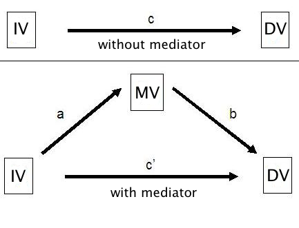
Sharma (2015) explains that Mediation analysis refers to the ‘estimation of the indirect effect of X on Y through an intermedi­ary mediator variable M causally located between X and Y (i.e., a model of the form X → M → Y)’. Or, as the graphic below describes IV → MV → DV.

This is exactly what they were looking to do. There were some complications however, they wanted the outcome variable to be modelled as a Poisson count of level of hallucination severity, the mediator was a binary indicator of abuse and the explanatory variable was also a binary indicator of whether the individual had an imaginary childhood friend. There were additional categorical control variables of gender and income.

Finding an appropriate model

Mediation analysis has a long history. A version of mediation analysis was outlined by Sewall Wright in 1934. As is often the case with statistical methods, although extremely clever people were able to demonstrate the possibility of a method several generations ago, this is unfortunately not equivalent to making the method accessible to those of lesser mathematical knowledge. Indeed, it is only in the last decades that the application of mediation analysis has expanded in fields such as psychology. This has been contingent on the growth of computing power along with software which renders these tools accessible to applied analysts. Even given current computer power and the ability of standard statistical software to handle mathematical models of increasing complexity, Mediation analysis has only relatively recently been absorbed into the most commonly used statistical packages.

R is very versatile and can handle a substantial range of data and models via recently released packages such as mediation:R. Those involved in statistical analysis know that R is a fantastically powerful software. The main drawback is that it requires a relatively high threshold of user knowledge to work in the environment. Stata comes somewhere between SPSS and R. To undertake analysis Stata requires more of a learning curve than SPSS but offers superior functionality and modelling capability. It offers less versatility or modelling capability than R, but nevertheless offers a wide variety of possibilities that are likely to meet the needs of most social-scientists.

Mediation:R would certainly do what we needed, but my experience as an analyst in R is that running into a problem in the package leads to substantial project delay. The knowledge threshold that R requires is comparatively high so that overcoming problems demands substantial outlays of time and mental capacity. This is not in itself an issue, but sometimes you have time to spend, and sometimes you need a result! My colleagues wanted the final piece of analysis for their paper.

A presentation by Grotta and Bellocco provided the solution in Stata. The presentation outlined several approaches to Mediation analysis including the PARAMED module. PARAMED enables Mediation analysis of categorical dependent variables such as our Poisson outcome. Checking the documentation that accompanied the installed module it allowed for exactly the model my colleagues needed. It also turned out that the PARAMED module is based on SAS and SPSS macros for running Mediation. Therefore the PARAMED functionality has equivalent in both SAS and SPSS.

I cannot claim to be a deep expert in SPSS but that is the package the team were working in. They were taking a look at the SPSS package PROCESS. I understand that the SPSS PROCESS package, has been written to allow Mediation analysis and version 3 handles categorical dependent variables. The developer of the PROCESS macro points to their book, Introduction to Mediation, Moderation, and Conditional Process Analysis for those interested in using this. Although it looks as though the analysis would be possible in PROCESS I have not yet found an instantiation, but there may well be one in the book.

It is apparent that functionality to undertake the modelling required is generally available. Stata is my preferred package and an example of a Mediation analysis in Stata is given below.

Analysis

The analysis used Stata 15. Variables specified in the analysis are listed below. The variable names are somewhat esoteric, sorry about that:

• UHRSUMPER is the count measure of hallucination
• ICTWOWAY is the binary measure of imaginary childhood companion (described as CIC status – childhood imaginary companion)
• SUMADVERSITY2WAY is the binary indicator of abuse
• Income is in three categories
• Male is binary men and women

The first thing I did was to install PARAMED and check the documentation, help files.

ssc install paramed
help paramed

I tried various model specifications, starting most simply.

The Stata code below specifies the full model:

paramed UHRSUMPER, avar(ICTWOWAY) mvar(SUMADVERSITY2WAY) cvars(under10k ten_25k  male) a0(0) a1(1) m(1) yreg(poisson) mreg(logistic) nointer boot seed(1234)

paramed invokes the paramed routine in Stata, yreg(poisson) specifies that the dependent variables is a count, mreg(logistic)specifies the mediator as binary. cvars(under10k ten_25k male) are dummy categories for the dummy variables of sex and income. The code a0(0) a1(1) m(1) specifies levels of the explanatory variable and the mediator. boot specifies whether a bootstrap procedure should be performed to compute bias-corrected bootstrap confidence intervals and seed specifies the seed for the bootstrap.

Mediation results output from Stata

	Estimate	Std Err	P>|z|	Lower 95% confidence Interval	Upper 95% confidence Interval
cde	1.253955	.10531446	0.032	1.0200853	1.5414429
nde	1.253955	.10531446	0.032	1.0200853	1.5414429
nie	1.088400	.03164556	0.007	1.0229427	1.158046
mte	1.3648047	.10552532	0.003	1.1098021	1.6784

mte=Total effect, nde=Natural direct effect, nie=Natural indirect effect

It was reported in the paper, ‘The relationship between CIC status and hallucination symptoms was mediated by childhood adversity where the total effect was significant (Estimate = 1.36, CI, 1.11 to 1.68) p = .003, as well as the natural direct effect (Estimate = 1.25, CI, 1.02 to 1.54) p = .032, and the natural indirect effect (Estimate = 1.09, CI, 1.02–1.16) p = .007.’

Conclusions

This blog has discussed some options available to undertake Mediation analyses in packages SPSS, R and Stata. An example of a potentially problematic Mediation analysis of a Poisson outcome has been outlined and it is shown that Stata was able to handle a tricky model like this via the user written program, PARAMED. In addition to giving readers an insight into options available to those interested in Mediation analysis the blog provides an opportunity to give due credit to the authors of the PARAMED module, Richard Emsley and Hanhua Liu. Unfortunately the journal that published the research article would not allow the inclusion of the reference for the PARAMED module, although we were able to name check the module in the text of the article. I have uploaded a pre-publication version of the paper with the reference attached and the full reference is provided below. Thank you Professor Emsley and Dr Hanhua Liu.

The co-auhthors on the research article are, Paige E. Davis, York St. John University, Lisa A. D. Webster, Leeds Trinity University, Charles Fernyhough Durham University, Helen J. Stain Leeds Trinity University Susanna Kola-Palmer University of Huddersfield.

**

Richard Emsley & Hanhua Liu, 2013. “PARAMED: Stata module to perform causal mediation analysis using parametric regression models,” Statistical Software Components S457581, Boston College Department of Economics, revised 26 Apr 2013.

A Categorical Can of Worms III

Examining categorical interactions in logit models using Marginal estimates and Marginsplot

Kevin Ralston 2018, York St John University

Introduction

This post is the third in a series of blogs which examine parameterisations of interactions in logit models. The first post outlined the generic, ‘conventional’ approach to including categorical interactions in logit models. The second post outlined an alternative specification of a categorical interaction in a logit. The current post outlines the application of marginal estimates and the marginsplot graph in the examination of categorical interactions in logit models.

Marginal estimates

Marginal estimates of categorical data are now part of the standard tool box in sociological research outputs. Margins produce estimates which have a ready interpretation. This is helpful because, as we have seen, working out what a model is showing us when an interaction is included is not straightforward. Williams (2017) explains what a marginal probability shows us in a logit model:

In the logit marginal results report the probability that a category is in the category coded 1 on the outcome. The MEM [marginal effect at means] for categorical variables therefore shows how P(Y=1) changes as the categorical variable changes from 0 to 1, holding all other variables at their means.

quietly logit class3 i.sex##i.ft i.qual c.age
margins i.sex#i.ft,

To produce marginal estimates at means we will estimate the basic model we have specified previously. We then follow this with a new line of code which includes the margins command, along with the variables included in the interaction. The quietly command here tells Stata not to produce the output for the model (we’ve seen it already).

Table1, Stata output, marginal estimates at means for an interaction from a logistic regression modelling membership of social class III, including independent variables sex, has a qualification, working full-time or part-time and age, also an interaction between age and working FT/PT. Source is GHS 1995, teaching dataset

In this case the margins are interpreted as the probability that each of the categories is in social class III at the average value (mean) of the other variables included in the model.

A standard criticism of marginal estimates at means is that the average value at which the estimates are calculated may have no substantive meaning. For example this model includes a categorical measure of whether an individual has qualifications, or not. By coincidence this variable is balanced close to 50% in each category. In a model including say, 30% with no qualifications the average marginal probabilities would be computed for an individual with 30% no qualification. In this model the margins are for an individual with ~50% no qualifications. This is problematic because we are referring to discrete categories. Someone with 50% no-qualifications cannot exist.

quietly logit class3 i.sex##i.ft i.qual c.age
margins i.sex#i.ft, at(qual=1) post,

It is also possible to estimate the marginal at a specific value of independent variables, such as qualifications. These have been described as adjusted predictions or predictive margins. This may be preferred. This is the specification I prefer as it offsets the criticism made above. It does not however mean that anyone in the data necessarily occupies the combination of categories in the model. There may still be no part time male workers with no-qualifications at the mean age of the sample. If there were we would expect them to have a probability of occupying social class III of .178 (quite low, closer to 0 than 1).

Table2, Stata output, adjusted predictions for an interaction from logistic regression modelling membership of social class III, including independent variables sex, has a qualification, working full-time or part-time and age, also an interaction between age and working FT/PT. Source is GHS 1995, teaching dataset

Marginsplot

The margins command has a neat graphing functionality.

Figure1, is a graphic of the marginal probability at means of being in social class III for the working full-time, part-time and sex interaction. The code for this is reported below.

logit class3 i.ft##i.sex i.qual c.age

       margins i.ft#i.sex,

             marginsplot , name(g2, replace) scheme(s1mono) ///

                    title (“Margins of ft/pt working and sex interaction”) ///

                    subtitle(“Outcome: member of social class III”) ///

                    legend(pos(7) ring(0)) ///

                    xtitle(“”) ytitle(“”) ///

                    xlabel(,angle(45))  ///

                    caption(“Source: GHS 95 teaching dataset”)   

 

To produce this graph you might notice I switched the position of the ft and sex dummy variables in the model. The graphical specification seems more sensible depicting ft/pt on the x-axis and depicting the difference within and between men and women. Maybe I should switch all the models so they are consistent. I had originally included sex in the model first for two reasons. Firstly, people have a biological sex and a socially constructed gender which influences their experience and choices, before they have a full time or part time job. Secondly, gendered occupational segregation is the area of substantive interest.

Building an analysis is an iterative process. There are good reasons to include sex before ft in the model, but in this case the interaction is presented more sensibly when organised i.ft##i.sex. Constructing an analysis often involves making small decisions and trade-offs like this.

Conclusion

In conclusion, I would suggest anyone fitting categorical interactions in logit models should both apply and report the marginal estimates. These have ready and relatively straightforward interpretations. They are certainly more intuitive than the interpretation of the results of a categorical interaction output in Stata applying a conventional interaction in a logit model.

Suggested reference should this post be useful to your work:

Ralston, K. 2018. A categorical can of worms III: Examining categorical interactions in logit models using Marginal estimates and Marginsplot. The Detective’s Handbook blog, Available at: thedetectiveshandbook.wordpress.com/2018/10/15/a-categorical-can-of-worms-iii/[Accessed: 15 October 2018].

 

Stata 15 Dynamic Documents: ‘.do files on steroids’

Roxanne Connelly, University of Warwick

Currently the transparency of social science research is poor, particularly in sociology. We tend to place little emphasis on undertaking research in a manner that would allow other researchers to repeat it, and approaches to sharing details of the research process are ad hoc and rarely used. To improve the transparency and reproducibility of sociological research I believe a step-change is required, not only the way we present the results of our research, but in the research process. Producing documentation for replication throughout the research process seems to be a key way in which we can move transparency from being an afterthought in the research process to being front and centre in our research conduct.

Building research transparency into the research process is not new, and borrows from the principles of literate programming introduced by Knuth (1992) in the field of computing science. Literate programming involves the weaving of narratives directly into live computation, interleaving text and documentation (beyond simple comments) with code and results to construct complete and transparent computations. The goal is to explain to humans, rather than machines, in natural language, what processes are being undertaken. The idea of literate programming has been taken up within the scientific computing community as a means to share self-documenting reproducible workflows but is very rarely implemented in sociology.

There are some packages available that can facilitate this type of literate programming for social science research. A notable example is Jupyter Notebooks, a web-based application that supports literate programming in a wide variety of languages (over 50 at present), including data analysis languages widely used for longitudinal social science research (i.e. R and Stata). Jupyter notebooks can run code from different computer programs in a language agnostic environment and can incorporate text and images. These notebooks can be shared and researchers can re-run the notebook and examine the results for themselves. An introduction to Jupyter Notebooks is available here. I am a big fan of Jupyter Notebooks, but currently an important drawback of this application is that it is difficult to install and there is a steep learning curve to get it working, particularly for those of us with limited computing science skills.

There are other packages available within specific statistical computing software environments that allow the combination of code, outputs and free text, e.g. Markdown and KnitR within R, or MarkDoc and Weaver in Stata. My main package is Stata so I was very excited to hear that their latest release (Stata 15) incorporates the capacity to create dynamic documents using Markdown. This allows you to mix Markdown with Stata commands and create a document that interweave the commands, output and text. Stata describes this as ‘a do-file on steroids.’

This blog provides an initial demonstration of Stata’s dynamic documents in action, and may serve as a useful start-up guide for some. I may add another blog once I have used it for the complete workflow of a real piece of data analysis. Here I describe the use of dyndoc which turns a plain text document into an HTML document, there is also putdocx (to create word documets) and putpdf (to create PDF files) but I have not looked at these yet.

Using dynamic documents is straightforward. First you create a plain text file containing the text you want to contain in the document along with the code. This file can include standard Markdown to create text formatting (e.g. bold, italics). When you have completed this file you run the dyndoc command (shown below) and your plain text file will be converted into an HTML document. You could then convert this to a PDF document using an HTML to PDF converter.

. dyndoc filename.txt, replace

To incorporate Stata code and output you use ‘tags’ in the plain text file which indicate whether the commands should appear in the document or not, or whether the output should appear in the document or not. To get the document formatted nicely you need to download the stylesheet ‘stmarkdown.css’ and the file ‘header.txt’ and save them in your working directory.

Here is my plain text file: blogexample

Here is the file that is produced by dyndoc (saved as a pdf to post): blogexamplehtml2pdf

I am really impressed with dyndoc, it was super quick to learn and provides a really straightforward way to improve the reproducibility of your work. Right now I anticipate that I will use it to create a document that can be attached as supplementary materials to journal publications. A dyndoc would greatly surpass a log file or .do file as a reader friendly way to present the complete workflow of a piece of research. Of course the effectiveness of a dyndoc for enabling reproducibility also requires the researcher to put the work in to provide sufficient annotation and description throughout the file. But if the dyndoc is cultivated throughout the research process this could be relatively painless.

There may be more eloquent ways to make use of dynamic documents in Stata and I am sure I will pick up more tricks as I use this more. I welcome comments from more experienced users of dyndoc!

A categorical can of worms: Examining interactions in logit models in Stata

Kevin Ralston, University of Edinburgh, 2017

1. The ‘conventional’ categorical by categorical interaction

Introduction

This post is the first of a series looking at interactions in non-linear models. This is a subject I have been thinking about for a while. It is an important issue for sociology, where we are often interested in substantively interesting categories and limited dependent variables. This series of posts is intended as a practical introduction to the issue and aimed at those new to thinking about such things.

There is a broad literature discussing interactions in logit/probit models. This is spread across a variety of publications and forums. Drawing on this I have summarised several strategies for examining interactions in a working paper which is currently circa 5000 words and growing. I had originally intended to present a comprehensive blog on these methods but the subject and its treatment is too large and detailed for a single blog!

As an alternative I will write a series of posts summarising methods for specifying and examining interactions. This is likely to include calculating ‘marginal effects’, cross-partial derivatives, the linear probability model and models reporting odds ratios. I hope it proves useful for some to draw this literature together in an introductory way. The more technical literature underlying the posts will be provided in references.

It may not be obvious that the interpretation of an interaction included in a logit model is not the same as an interaction included in an ordinary least squares model (OLS). In this first instance this blog outlines what may be considered a ‘conventional’ specification of a categorical by categorical interaction and how it may be interpreted.

Data

Suppose we are interested in looking at the relationship between those in social class III of Registrar Generals social class (RGSC) and various independent variables.

The data used are from the General Household Survey 1995 teaching dataset (Cooper and Arber 2000). This is available to download from the UK data archive. The dependent variable is dichotomous controlling for whether a case is recorded as being in social class III or not (Table 1). Independent variables are also dichotomised and include whether an individual has qualifications or no qualifications; is working full-time or part-time and their age.

Table 1, frequencies of distributions of variables of interest by whether an individual is a man or a woman, including chi-square and phi levels
	% (n)		Chi-square p-value	Phi
	Men	Women
Not class III	60 (1043)	40 (698)	0.00	0.31
Class III	23 (126)	77 (413)
Qualification	52 (924)	48 (857)	0.27	0.02
No Quals	49 (245)	51 (254)
Part-time	16 (97)	84 (499)	0.00	-0.42
Full-time	64 (1072)	36 (612)
			Min	max	sd
Mean age men	40		16	69	12
Mean age women	39		16	67	12
n=	1169	1111
Source, General Household Survey 1995

 Although this is an example from a teaching dataset, chosen because it illustrates certain patterns and relationships in the data, there could easily be reasons why a researcher would look to model such relationships. One might be if a researcher were interested in processes or outcomes related to gendered occupational segregation. RGSC is an older measure and might not be the first choice for many sociologists. It is a measure still widely used in public health research, and there may be reasons to compare RGSC with other occupationally based social class measures.

The sample comprises of a complete case analysis of everyone in the data who are over 16 and non-missing.

Analysis

Occupational position changes across the life course as people often transition from perhaps less secure low skilled employment in their youth, to career positions post education. In this respect these analyses are non-conventional in that they include everyone over 16 who is in work.

Given this wide age range we shall include age in our model. In a more formal piece of research we would consider whether such a large age range is appropriate. It would not be usual to consider the occupational position of 16 year olds in the same model as 40 year olds or 59 year olds, because those who are older have qualifications and experience and more time to position themselves in the labour force. It is important to be aware of such issues and to consider them carefully in undertaking analysis. In the current analyses we will choose to ignore these important issues and concentrate on interactions in models.

Basic Model

Below is the Stata output for a logistic regression model measuring the association between the independent variables described above and membership of social class III. The code to produce the model is also given. In Sata the i. prefix specifies that the variable is a factor (categorical) variable, the c. prefix for continuous, metric variables.

logit class3 i.sex i.qual i.ft c.age

Table 1, Stata output, logistic regression modelling membership of social class III, including independent variables sex, has a qualification, working full-time or part-time and age. Source is GHS 1995, teaching dataset

All of the variables included suggest significant associations. Age at the p<=0.04 level and all others at <=0.001 level.

The coefficients associated with the independent variables express the log-odds of being in social class III. For the categorical variables this is compared to a base category. For example, for ‘sex’ the base category is men. The coefficient reported for sex expresses the log-odds that women are in class III compared to men. For qualification the base category is those with a qualification and the coefficient expresses the log-odds of being in class III for those who have no qualifications, compared to those who have qualifications. Age has been included in the model as a linear metric variable. The coefficient reported for this shows the log-odds of being in class III for a one year increase in age.

The models show that women are more likely to be in social class III compared to men. Those with no-qualifications are less likely to be in class III than those with qualifications. People in social class III are less likely to work full time than part time. It can also be seen that those who are older are less likely to be in social class III.

A categorical by categorical interaction: Model with an interaction between sex and full-time/part-time working, conventionally expressed

It is generally known that, on average, women are more likely to be employed part-time than men. We can include an interaction between sex and employment in the model to represent this.

logit class3 i.sex##i.ft i.qual c.age 

Table 2, Stata output, logistic regression modelling membership of social class III, including independent variables sex, has a qualification, working full-time or part-time and age, also an interaction between sex and working FT/PT. Source is GHS 1995, teaching dataset

We can specify an interaction between variables in a number of ways. Using a double hashtag (##) between the variables generates a model output of what may be considered a ‘conventional’ interaction. Stata describes the # command as representing an interaction and the double hashtag ## as representing a factorial interaction[1].

The output this generates (Table2) is similar to the output produced in Table1. There is an additional term reported with a value related to the interaction (2. Female#FT). As before the coefficients express the log-odds associated with a category, compared to a base category. Things are a bit more complicated and confusing because the base category and contrast categories are now composites of the sex and part-time/full-time variable.

The values reported for the female category and the FT category now report a comparison with the group which is in the base category on both the variables included in the interaction. In the case of these analyses this is men who were employed part-time. The coefficient for females is the comparison between men working part-time and women working part-time. The coefficient for FT is the comparison between men working part-time and men working full-time.

Many researchers are familiar with OLS regression models. In OLS models an interaction term reports the partial derivative. Wikipedia describes this as ‘the function of two or more variables with respect to one variable, the other(s) being treated as constant’[2]. In logit (and probit) models, specified as log-odds, this is not what is reported by the interaction term.

Kohler and Kreuter (2009) tell us that the coefficient for the interaction term reports how much the association changes at different levels of the dependent variables. The coefficient for the interaction term here (in this case Female#FT) reports how much the association of sex changes when full time workers are considered instead of part-time workers. The term is reported as significant at p<=0.001 level. But this may not have substantive importance, given that the value is a value for a change between categories and not a contrast between dummy categories!

We know the base category is men working part time, because this is a composite of the two base categories of the sex and FT variable. Following Kholer and Kreuter (2009) we can do a bit of addition to derive values of terms associated with other comparisons of potential interest.

Examples:

1.  0.7+0.94= 1.64, if women working part-time have a 0.7 higher log-odds of being in social class III than men who are working part time then 1.64 is the comparison between women working full-time and men working full-time
2. -1.2+0.94= -0.26, -0.26 is the comparison between women working PT and women working FT, with women working FT less likely to be in social class III

The 0.7 in example 1, above, comes from the female coefficient in the model. It has been rounded from 0.6969, to 0.7. This is added to the interaction coefficient for Female#FT of 0.94 to get the value 1.64. Example 2 is derived similarly the -1.2 is taken from the value of the FT coefficient and added to the Female#FT of 0.94.

This can be checked by changing the specification and the reference categories in the model (Additional table 2). This is what I did to try to make sure the comparisons reported are correct! In practice this took several checks and re-checks before I was confident.

The likelihood ratio chi square test tells us the model with the interaction is a ‘better’ fit than the model without the interaction (see Additional table 1):

((-1109)-(- 1114))x2 = 10,

This is highly significant at 1 degree of freedom (p=0.0015).

It may be suggested that the specification given above is a ‘standard parameterisation’ (Royston and Sauerbrei 2012). I personally find modelling interactions specified in this manner to be opaque, in terms of their interpretation. Indeed, I find understanding the relationship described by an interaction takes time and effort to puzzle out.

Conclusion

This post has outlined the most basic approach to including a categorical by categorical interaction in a logit model.

In ordinary least squares models the interaction term reports the partial derivative. This is not what is reported for an interaction in a logit model specified as log-odds. The coefficient for the interaction term in the logit reports how much the association changes at different levels of the dependent variables. This can be quite difficult to think about and interpret.

Various alternatives to this ‘conventional’ model are available. Future posts in this series will outline several of these.

See:

A categorical can of worms II for an alternative specification of the interaction

A categorical can of worms III for the use of margins and Stata’s marginsplot in examining interactions

 

[1] http://www.stata.com/statalist/archive/2009-06/msg00945.html

[2] https://en.wikipedia.org/wiki/Partial_derivative

Suggested reference should this post be useful to your work:

Ralston, K. 2017. A categorical can of worms: Examining interactions in logit models in Stata. The Detective’s Handbook blog, Available at: https://thedetectiveshandbook.wordpress.com/2017/03/15/a-categorical-can-of-worms-examining-interactions-in-logit-models-in-stata/ [Accessed: 2 July 2018].

 

References

Cooper, H. and Arber, S. 2000. General Household Survey, 1995: Teaching Dataset. [data collection]. 2nd Edition.

Kohler, U. and Kreuter, F. 2009. Data Analysis Using Stata: Second Edition. College Station, Tx: Stata Press.

Royston, P. and Sauerbrei, W. 2012. Handling Interactions in Stata, especially with continuous predictors. . Available at: http://www.stata.com/meeting/germany12/abstracts/desug12_royston.pdf <accessed, 15/03/17>

Additional table 1, this provides an alternative descriptive table of variables, the models from tables 1 and 2 along with the likelihood ratio chi-square test

Additional table 2, this shows an alternative specification of the interaction and alters the reference categories to demonstrate associations at alternative levels of the interaction. These show values which match those calculated in example 1 and 2, above.