A categorical can of worms: Examining interactions in logit models in Stata

Kevin Ralston, University of Edinburgh, 2017

1. The ‘conventional’ categorical by categorical interaction

Introduction

This post is the first of a series looking at interactions in non-linear models. This is a subject I have been thinking about for a while. It is an important issue for sociology, where we are often interested in substantively interesting categories and limited dependent variables. This series of posts is intended as a practical introduction to the issue and aimed at those new to thinking about such things.

There is a broad literature discussing interactions in logit/probit models. This is spread across a variety of publications and forums. Drawing on this I have summarised several strategies for examining interactions in a working paper which is currently circa 5000 words and growing. I had originally intended to present a comprehensive blog on these methods but the subject and its treatment is too large and detailed for a single blog!

As an alternative I will write a series of posts summarising methods for specifying and examining interactions. This is likely to include calculating ‘marginal effects’, cross-partial derivatives, the linear probability model and models reporting odds ratios. I hope it proves useful for some to draw this literature together in an introductory way. The more technical literature underlying the posts will be provided in references.

It may not be obvious that the interpretation of an interaction included in a logit model is not the same as an interaction included in an ordinary least squares model (OLS). In this first instance this blog outlines what may be considered a ‘conventional’ specification of a categorical by categorical interaction and how it may be interpreted.

Data

Suppose we are interested in looking at the relationship between those in social class III of Registrar Generals social class (RGSC) and various independent variables.

The data used are from the General Household Survey 1995 teaching dataset (Cooper and Arber 2000). This is available to download from the UK data archive. The dependent variable is dichotomous controlling for whether a case is recorded as being in social class III or not (Table 1). Independent variables are also dichotomised and include whether an individual has qualifications or no qualifications; is working full-time or part-time and their age.

Table 1, frequencies of distributions of variables of interest by whether an individual is a man or a woman, including chi-square and phi levels
	% (n)		Chi-square p-value	Phi
	Men	Women
Not class III	60 (1043)	40 (698)	0.00	0.31
Class III	23 (126)	77 (413)
Qualification	52 (924)	48 (857)	0.27	0.02
No Quals	49 (245)	51 (254)
Part-time	16 (97)	84 (499)	0.00	-0.42
Full-time	64 (1072)	36 (612)
			Min	max	sd
Mean age men	40		16	69	12
Mean age women	39		16	67	12
n=	1169	1111
Source, General Household Survey 1995

 Although this is an example from a teaching dataset, chosen because it illustrates certain patterns and relationships in the data, there could easily be reasons why a researcher would look to model such relationships. One might be if a researcher were interested in processes or outcomes related to gendered occupational segregation. RGSC is an older measure and might not be the first choice for many sociologists. It is a measure still widely used in public health research, and there may be reasons to compare RGSC with other occupationally based social class measures.

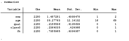
The sample comprises of a complete case analysis of everyone in the data who are over 16 and non-missing.

Analysis

Occupational position changes across the life course as people often transition from perhaps less secure low skilled employment in their youth, to career positions post education. In this respect these analyses are non-conventional in that they include everyone over 16 who is in work.

Given this wide age range we shall include age in our model. In a more formal piece of research we would consider whether such a large age range is appropriate. It would not be usual to consider the occupational position of 16 year olds in the same model as 40 year olds or 59 year olds, because those who are older have qualifications and experience and more time to position themselves in the labour force. It is important to be aware of such issues and to consider them carefully in undertaking analysis. In the current analyses we will choose to ignore these important issues and concentrate on interactions in models.

Basic Model

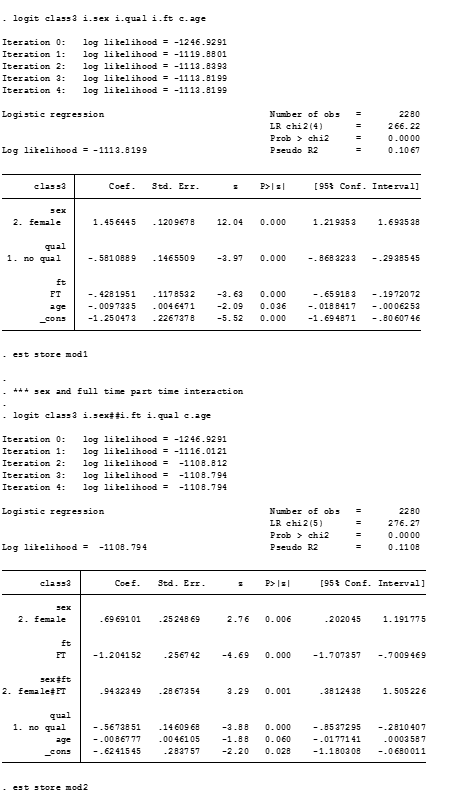
Below is the Stata output for a logistic regression model measuring the association between the independent variables described above and membership of social class III. The code to produce the model is also given. In Sata the i. prefix specifies that the variable is a factor (categorical) variable, the c. prefix for continuous, metric variables.

logit class3 i.sex i.qual i.ft c.age

Table 1, Stata output, logistic regression modelling membership of social class III, including independent variables sex, has a qualification, working full-time or part-time and age. Source is GHS 1995, teaching dataset

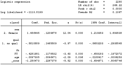
All of the variables included suggest significant associations. Age at the p<=0.04 level and all others at <=0.001 level.

The coefficients associated with the independent variables express the log-odds of being in social class III. For the categorical variables this is compared to a base category. For example, for ‘sex’ the base category is men. The coefficient reported for sex expresses the log-odds that women are in class III compared to men. For qualification the base category is those with a qualification and the coefficient expresses the log-odds of being in class III for those who have no qualifications, compared to those who have qualifications. Age has been included in the model as a linear metric variable. The coefficient reported for this shows the log-odds of being in class III for a one year increase in age.

The models show that women are more likely to be in social class III compared to men. Those with no-qualifications are less likely to be in class III than those with qualifications. People in social class III are less likely to work full time than part time. It can also be seen that those who are older are less likely to be in social class III.

A categorical by categorical interaction: Model with an interaction between sex and full-time/part-time working, conventionally expressed

It is generally known that, on average, women are more likely to be employed part-time than men. We can include an interaction between sex and employment in the model to represent this.

logit class3 i.sex##i.ft i.qual c.age 

Table 2, Stata output, logistic regression modelling membership of social class III, including independent variables sex, has a qualification, working full-time or part-time and age, also an interaction between sex and working FT/PT. Source is GHS 1995, teaching dataset

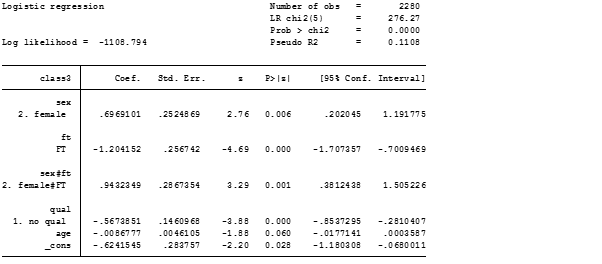
We can specify an interaction between variables in a number of ways. Using a double hashtag (##) between the variables generates a model output of what may be considered a ‘conventional’ interaction. Stata describes the # command as representing an interaction and the double hashtag ## as representing a factorial interaction[1].

The output this generates (Table2) is similar to the output produced in Table1. There is an additional term reported with a value related to the interaction (2. Female#FT). As before the coefficients express the log-odds associated with a category, compared to a base category. Things are a bit more complicated and confusing because the base category and contrast categories are now composites of the sex and part-time/full-time variable.

The values reported for the female category and the FT category now report a comparison with the group which is in the base category on both the variables included in the interaction. In the case of these analyses this is men who were employed part-time. The coefficient for females is the comparison between men working part-time and women working part-time. The coefficient for FT is the comparison between men working part-time and men working full-time.

Many researchers are familiar with OLS regression models. In OLS models an interaction term reports the partial derivative. Wikipedia describes this as ‘the function of two or more variables with respect to one variable, the other(s) being treated as constant’[2]. In logit (and probit) models, specified as log-odds, this is not what is reported by the interaction term.

Kohler and Kreuter (2009) tell us that the coefficient for the interaction term reports how much the association changes at different levels of the dependent variables. The coefficient for the interaction term here (in this case Female#FT) reports how much the association of sex changes when full time workers are considered instead of part-time workers. The term is reported as significant at p<=0.001 level. But this may not have substantive importance, given that the value is a value for a change between categories and not a contrast between dummy categories!

We know the base category is men working part time, because this is a composite of the two base categories of the sex and FT variable. Following Kholer and Kreuter (2009) we can do a bit of addition to derive values of terms associated with other comparisons of potential interest.

Examples:

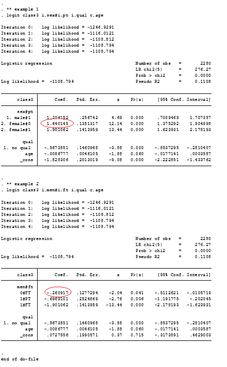
1.  0.7+0.94= 1.64, if women working part-time have a 0.7 higher log-odds of being in social class III than men who are working part time then 1.64 is the comparison between women working full-time and men working full-time
2. -1.2+0.94= -0.26, -0.26 is the comparison between women working PT and women working FT, with women working FT less likely to be in social class III

The 0.7 in example 1, above, comes from the female coefficient in the model. It has been rounded from 0.6969, to 0.7. This is added to the interaction coefficient for Female#FT of 0.94 to get the value 1.64. Example 2 is derived similarly the -1.2 is taken from the value of the FT coefficient and added to the Female#FT of 0.94.

This can be checked by changing the specification and the reference categories in the model (Additional table 2). This is what I did to try to make sure the comparisons reported are correct! In practice this took several checks and re-checks before I was confident.

The likelihood ratio chi square test tells us the model with the interaction is a ‘better’ fit than the model without the interaction (see Additional table 1):

((-1109)-(- 1114))x2 = 10,

This is highly significant at 1 degree of freedom (p=0.0015).

It may be suggested that the specification given above is a ‘standard parameterisation’ (Royston and Sauerbrei 2012). I personally find modelling interactions specified in this manner to be opaque, in terms of their interpretation. Indeed, I find understanding the relationship described by an interaction takes time and effort to puzzle out.

Conclusion

This post has outlined the most basic approach to including a categorical by categorical interaction in a logit model.

In ordinary least squares models the interaction term reports the partial derivative. This is not what is reported for an interaction in a logit model specified as log-odds. The coefficient for the interaction term in the logit reports how much the association changes at different levels of the dependent variables. This can be quite difficult to think about and interpret.

Various alternatives to this ‘conventional’ model are available. Future posts in this series will outline several of these.

See:

A categorical can of worms II for an alternative specification of the interaction

A categorical can of worms III for the use of margins and Stata’s marginsplot in examining interactions

 

[1] http://www.stata.com/statalist/archive/2009-06/msg00945.html

[2] https://en.wikipedia.org/wiki/Partial_derivative

Suggested reference should this post be useful to your work:

Ralston, K. 2017. A categorical can of worms: Examining interactions in logit models in Stata. The Detective’s Handbook blog, Available at: https://thedetectiveshandbook.wordpress.com/2017/03/15/a-categorical-can-of-worms-examining-interactions-in-logit-models-in-stata/ [Accessed: 2 July 2018].

 

References

Cooper, H. and Arber, S. 2000. General Household Survey, 1995: Teaching Dataset. [data collection]. 2nd Edition.

Kohler, U. and Kreuter, F. 2009. Data Analysis Using Stata: Second Edition. College Station, Tx: Stata Press.

Royston, P. and Sauerbrei, W. 2012. Handling Interactions in Stata, especially with continuous predictors. . Available at: http://www.stata.com/meeting/germany12/abstracts/desug12_royston.pdf <accessed, 15/03/17>

Additional table 1, this provides an alternative descriptive table of variables, the models from tables 1 and 2 along with the likelihood ratio chi-square test

Additional table 2, this shows an alternative specification of the interaction and alters the reference categories to demonstrate associations at alternative levels of the interaction. These show values which match those calculated in example 1 and 2, above.